R2 basic tutorial
In this tutorial you will learn how to use the Python API of R* codes (http://www.es.lancs.ac.uk/people/amb/Freeware/R2/R2.htm). Start by importing the Project master class from the API (Application Programming Interface).
1 Basics imports
Just import basic packages and the R2 API as a module (note : you will need to change the path for it, here we assume you launched the jupyter from inside the /examples/jupyter-notebook folder).
[1]:
%matplotlib inline
import warnings
warnings.filterwarnings('ignore')
import os
import sys
sys.path.append((os.path.relpath('../src'))) # add here the relative path of the API folder
testdir = '../src/examples/dc-2d/'
from resipy import Project
API path =  /media/jkl/data/phd/resipy/src/resipy
ResIPy version =  3.4.6
cR2.exe found and up to date.
R3t.exe found and up to date.
cR3t.exe found and up to date.
2 Create an ‘Project’ object, import data and plot pseudo section
The
Projectclass was referred to asR2class in older version of ResIPy.
The first step is to create an object out of the Project class, let’s call it k . This is the main object we are going to interact with. Then the second step is to read the data from a survey file. Here we choose a csv file from the Syscal Pro that contains resistivity data only. Note then when importing the survey data, the object automatically search for reciprocal measurements and will compute a reciprocal error with the ones it finds.
[2]:
k = Project(typ='R2') # create a Project object in a working directory (can also set using k.setwd())
k.createSurvey(testdir + 'syscal.csv', ftype='Syscal') # read the survey file
Working directory is: /media/jkl/data/phd/resipy/src/resipy
clearing dirname
308/344 reciprocal measurements found.
0 measurements error > 20 %
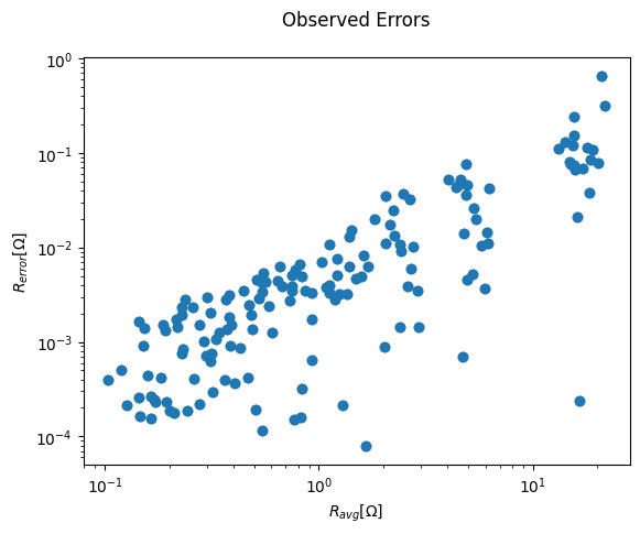
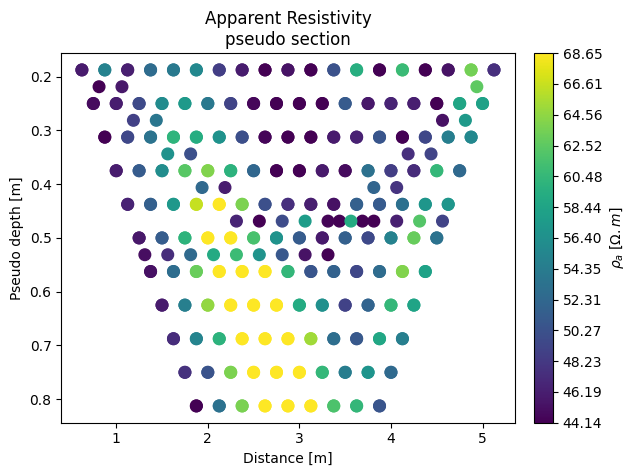
We can plot the pseudosection and display errors based on reciprocal measurements.
[3]:
k.showPseudo()
k.showError() # plot the reciprocal errors

3 Data filtering
Below are a few examples of data filtering routines that can be used: - k.filterUnpaired() to remove unpaired measurements (so measurements with no reciprocal) -> those could be dummy measurements in a dipole-dipole configuration - k.filterElec([5]) to remove a specific electrode (e.g. here all quadrupoles with electrode 5 are deleted) - k.filterRecip(20) to remove measurements based on their relative reciprocal error (e.g. all quadrupoles with a reciprocal error > 20% are
discarded). More advanced data filtering can be achieved using the filterData() method from the Survey class. This method allows to filter out specific quadrupoles. An interactive version of it can be access using the filterManual() method which produces an interactive pseudo-section in the UI.
[4]:
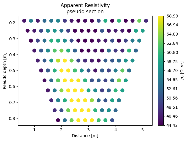
k.filterUnpaired()
k.showPseudo() # this actually removed the dummy measurements in this dipole-dipole survey (added for speed optimization)
removeUnpaired:filterData: 36 / 344 quadrupoles removed.
[5]:
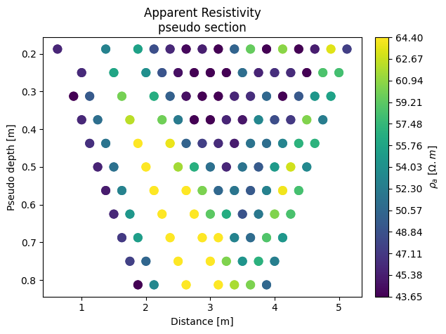
k.filterElec([5]) # remove all quadrupoles associated with electrode 5
k.showPseudo()
filterData: 48 / 308 quadrupoles removed.
48 measurements removed!

[6]:
k.filterRecip(percent=20) # in this case this only removes one quadrupoles with reciprocal error bigger than 20 percent
k.showPseudo()
0 measurements with greater than 20.0% reciprocal error removed!
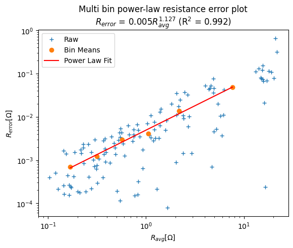
4 Fitting an error model
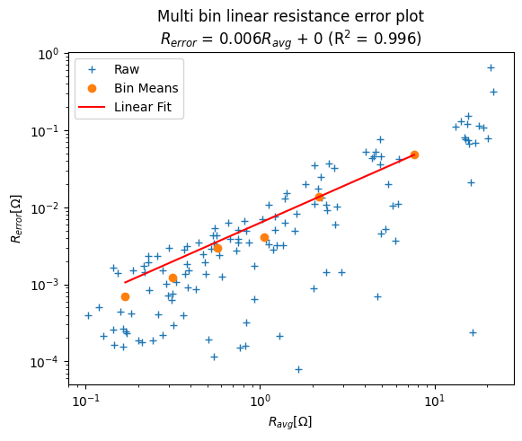
Different errors models are available to be fitted for DC data: - a simple linear model: k.fitErrorLin() - a power law model: k.fitErrorPwl() - a linear mixed effect model: k.fitErrorLME() (on Linux only with an R kernel installed) Each of those will create a new error column in the Survey object that will be used in the inversion if k.err = True.
[7]:
k.fitErrorLin()
Error model is R_err = 0.006*R_avg + 0 (R^2 = 0.996)
[8]:
k.fitErrorPwl()
Error model is R_err = 0.005 R_avg^1.127 (R^2 = 0.992)
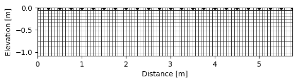
5 Mesh
Two types of mesh can be created in 2D: - a quadrilateral mesh (k.createMesh('quad')) - a triangular mesh (k.createmesh('trian')) For 3D, only tetrahedral mesh can be created using k.createMesh('tetra').
[9]:
k.createMesh(typ='quad') # generate quadrilateral mesh (default for 2D survey)
k.showMesh()
Creating quadrilateral mesh...done (3306 elements)
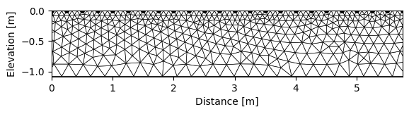
[10]:
k.createMesh('trian', show_output=False) # this actually call gmsh.exe to create the mesh
k.showMesh()
Creating triangular mesh...done (1642 elements)
7 Inversion
The inversion takes place in the specify working directory of the R2 object specified the first time the k = R2(<workingDirectory>) is called. It can be changed after by using k.setwd(<newWorkingDirectory>). The parameters of the inversion are defined in a dictionnary in k.param and ca be changed manually by the user (e.g. k.param['a_wgt'] = 0.01. All parameters have a default values and their names follow the R2 manual. The .in file is written automatically when the
k.invert() method is called.
[11]:
k.param['data_type'] = 1 # using log of resistitivy
k.err = True # if we want to use the error from the error models fitted before
k.invert() # this will do the inversion
Writing .in file and protocol.dat... done

--------------------- MAIN INVERSION ------------------


 >> R  2    R e s i s t i v i t y   I n v e r s i o n   v4.10 <<

 >> D a t e : 03 - 12 - 2023
 >> My beautiful survey
 >> I n v e r s e   S o l u t i o n   S e l e c t e d <<
 >> Determining storage needed for finite element conductance matrix
 >> Generating index array for finite element conductance matrix
 >> Reading start resistivity from res0.dat
 >> R e g u l a r i s e d   T y p e <<
 >>   L i n e a r    F i l t e r    <<
 >> L o g - D a t a   I n v e r s i o n <<
 >> N o r m a l   R e g u l a r i s a t i o n <<
 >> D a t a   w e i g h t s   w i l l   b e  m o d i f i e d <<
 >> D a t a   w e i g h t   t o   b e   r e a d   f r o m   d a t a   f i l e <<


 Processing dataset   1


 Measurements read:   130     Measurements rejected:     0
   Geometric mean of apparent resistivities:  0.52480E+02

 >> Total Memory required is:          0.002 Gb

   Iteration   1
     Initial RMS Misfit:       125.18       Number of data ignored:     0
     Alpha:        4290.693   RMS Misfit:        7.62  Roughness:        1.683
     Alpha:        1991.563   RMS Misfit:        6.52  Roughness:        2.389
     Alpha:         924.402   RMS Misfit:        5.60  Roughness:        3.498
     Alpha:         429.069   RMS Misfit:        4.92  Roughness:        5.145
     Alpha:         199.156   RMS Misfit:        4.61  Roughness:        7.204
     Alpha:          92.440   RMS Misfit:        4.60  Roughness:        9.502
     Alpha:          42.907   RMS Misfit:        5.47  Roughness:       12.258
     Step length set to   1.00000
     Final RMS Misfit:        4.60
     Updated data weights

   Iteration   2
     Initial RMS Misfit:         3.45       Number of data ignored:     0
     Alpha:          52.960   RMS Misfit:        1.09  Roughness:       11.091
     Alpha:          24.582   RMS Misfit:        0.78  Roughness:       13.255
     Step length set to   1.00000
     Final RMS Misfit:        0.78
     Final RMS Misfit:        1.03

 Solution converged - Outputing results to file

 Calculating sensitivity map


 Processing dataset   2


 End of data:  Terminating
1/1 results parsed (1 ok; 0 failed)
All ok
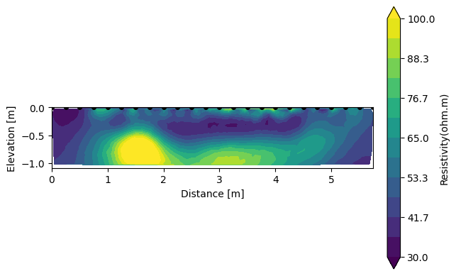
8 Results visualisation and post-processing
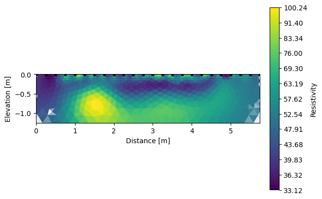
Results can be show with k.showResults(). Multiple arguments can be passed to the method in order rescale the colorbar bar, view the sensitivity or not, change the attribute or plot contour. The errors from the inversion can also be plotted using either k.pseudoError() or k.showInvError().
[12]:
k.showResults(attr='Resistivity(ohm.m)', sens=False, contour=True, vmin=30, vmax=100)
/media/jkl/data/phd/resipy/doc/gallery/../../src/resipy/meshTools.py:1487: MatplotlibDeprecationWarning: The collections attribute was deprecated in Matplotlib 3.8 and will be removed two minor releases later.
  for col in cont.collections:
/media/jkl/data/phd/resipy/doc/gallery/../../src/resipy/Project.py:4136: MatplotlibDeprecationWarning: The collections attribute was deprecated in Matplotlib 3.8 and will be removed two minor releases later.
  colls = mesh.cax.collections if contour == True else [mesh.cax]
[13]:
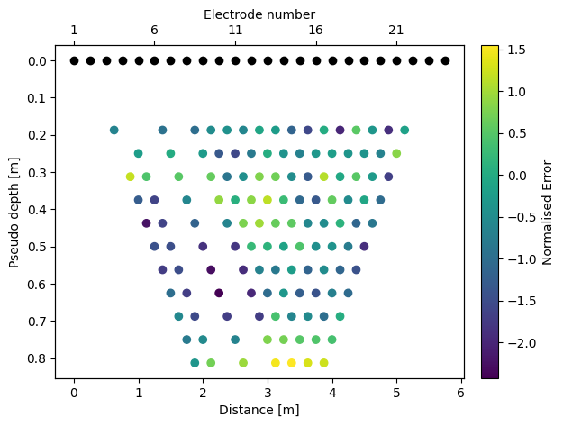
k.showPseudoInvError() # allow to see if some electrodes get higher error
[14]:
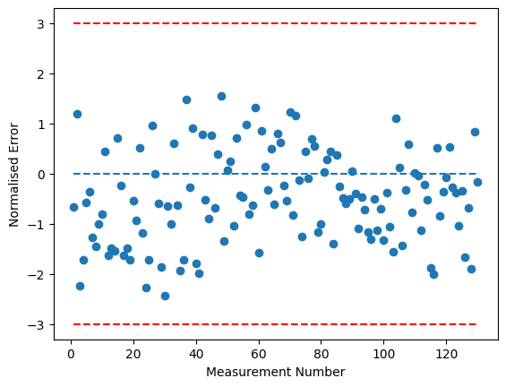
k.showInvError() # all errors should be between -3 and 3
In a nutshell
Below is a minimal example which imports the data, plots a pseudo section and inverts using all default parameters.
[15]:
k = Project(typ='R2') # create an Project object in a working directory (can also set using k.setwd())
k.createSurvey(testdir + 'syscal.csv', ftype='Syscal') # read the survey file
k.showPseudo() # plot pseudo section
k.invert(iplot=True) # does the inversion (generate quand mesh and use default R2.in settings)
Working directory is: /media/jkl/data/phd/resipy/src/resipy
clearing dirname
308/344 reciprocal measurements found.
0 measurements error > 20 %
Creating triangular mesh...done (1786 elements)
Writing .in file and protocol.dat... done

--------------------- MAIN INVERSION ------------------


 >> R  2    R e s i s t i v i t y   I n v e r s i o n   v4.10 <<

 >> D a t e : 03 - 12 - 2023
 >> My beautiful survey
 >> I n v e r s e   S o l u t i o n   S e l e c t e d <<
 >> Determining storage needed for finite element conductance matrix
 >> Generating index array for finite element conductance matrix
 >> Reading start resistivity from res0.dat
 >> R e g u l a r i s e d   T y p e <<
 >>   L i n e a r    F i l t e r    <<
 >> L o g - D a t a   I n v e r s i o n <<
 >> N o r m a l   R e g u l a r i s a t i o n <<
 >> D a t a   w e i g h t s   w i l l   b e  m o d i f i e d <<


 Processing dataset   1


 Measurements read:   190     Measurements rejected:     0
   Geometric mean of apparent resistivities:  0.52987E+02

 >> Total Memory required is:          0.003 Gb

   Iteration   1
     Initial RMS Misfit:        28.73       Number of data ignored:     0
     Alpha:         430.648   RMS Misfit:        1.97  Roughness:        1.966
     Alpha:         199.889   RMS Misfit:        1.54  Roughness:        2.907
     Alpha:          92.780   RMS Misfit:        1.23  Roughness:        4.065
     Alpha:          43.065   RMS Misfit:        1.02  Roughness:        5.479
     Alpha:          19.989   RMS Misfit:        0.90  Roughness:        7.232
     Step length set to   1.00000
     Final RMS Misfit:        0.90

 Cannot fit quadratic through step lengths
     Final RMS Misfit:        0.90

 Solution converged - Outputing results to file

 Calculating sensitivity map


 Processing dataset   2


 End of data:  Terminating
1/1 results parsed (1 ok; 0 failed)
All ok
[ ]: