Forward modelling
In this tutorial, we will see how to use pyR2 API to do forward modelling.
[1]:
import warnings
warnings.filterwarnings('ignore')
import os
import sys
sys.path.append((os.path.relpath('../src'))) # add here the relative path of the API folder

import numpy as np # numpy for electrode generation
from resipy import Project
API path =  /media/jkl/data/phd/resipy/src/resipy
ResIPy version =  3.4.6
cR2.exe found and up to date.
R3t.exe found and up to date.
cR3t.exe found and up to date.
[2]:
k = Project(typ='R2') # create R2 object
Working directory is: /media/jkl/data/phd/resipy/src/resipy
clearing dirname
First we need to design some electrodes. We will use numpy functions for this.
[3]:
elec = np.zeros((24,3))
elec[:,0] = np.arange(0, 24*0.5, 0.5) # with 0.5 m spacing and 24 electrodes
k.setElec(elec)
print(k.elec)
   label     x    y    z  remote  buried
0      1   0.0  0.0  0.0   False   False
1      2   0.5  0.0  0.0   False   False
2      3   1.0  0.0  0.0   False   False
3      4   1.5  0.0  0.0   False   False
4      5   2.0  0.0  0.0   False   False
5      6   2.5  0.0  0.0   False   False
6      7   3.0  0.0  0.0   False   False
7      8   3.5  0.0  0.0   False   False
8      9   4.0  0.0  0.0   False   False
9     10   4.5  0.0  0.0   False   False
10    11   5.0  0.0  0.0   False   False
11    12   5.5  0.0  0.0   False   False
12    13   6.0  0.0  0.0   False   False
13    14   6.5  0.0  0.0   False   False
14    15   7.0  0.0  0.0   False   False
15    16   7.5  0.0  0.0   False   False
16    17   8.0  0.0  0.0   False   False
17    18   8.5  0.0  0.0   False   False
18    19   9.0  0.0  0.0   False   False
19    20   9.5  0.0  0.0   False   False
20    21  10.0  0.0  0.0   False   False
21    22  10.5  0.0  0.0   False   False
22    23  11.0  0.0  0.0   False   False
23    24  11.5  0.0  0.0   False   False
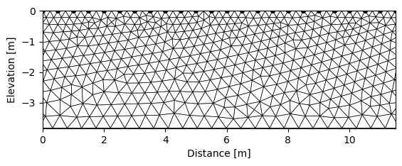
Now let’s create a mesh.
[4]:
k.createMesh(typ='trian', show_output=False, res0=200) # let's create the mesh based on these electrodes position
k.showMesh()
Creating triangular mesh...done (1887 elements)
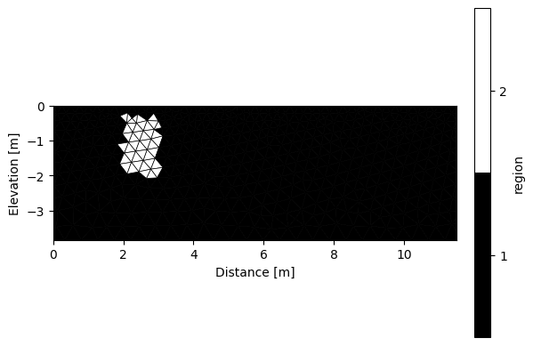
Based on this mesh, we can defined regions and assign them conductivities. There is an interactive way to do it when working outside of the jupyter notebook in interactive mode or GUI. Here we will see the pure API based way to do it using R2.addRegion().
[5]:
help(k.addRegion) # to display the help of the method
Help on method addRegion in module resipy.Project:

addRegion(xz, res0=100, phase0=1, blocky=False, fixed=False, ax=None, iplot=False) method of resipy.Project.Project instance
    Add region according to a polyline defined by `xz` and assign it
    the starting resistivity `res0`.

    Parameters
    ----------
    xz : array
        Array with two columns for the x and y coordinates.
    res0 : float, optional
        Resistivity values of the defined area.
    phase0 : float, optional
        Read only if you choose the cR2 option. Phase value of the defined
        area in mrad
    blocky : bool, optional
        If `True` the boundary of the region will be blocky if inversion
        is block inversion.
    fixed : bool, optional
        If `True`, the inversion will keep the starting resistivity of this
        region.
    ax : matplotlib.axes.Axes
        If not `None`, the region will be plotted against this axes.
    iplot : bool, optional
        If `True` , the updated mesh with the region will be plotted.
[6]:
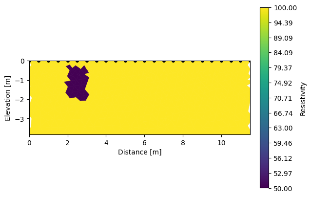
k.addRegion(np.array([[2,-0.3],[2,-2],[3,-2],[3,-0.3],[2,-0.3]]), 50, iplot=True)
# first specify the path of the region and then its resistivity value in Ohm.m
We then need to define the sequence that we will use. We can easily create a dipole-dipole sequence using R2.createSequence() or import one using R2.importSequence().
[7]:
help(k.createSequence) # don't hersitate to use the help to know more about each method
Help on method createSequence in module resipy.Project:

createSequence(params=[('dpdp1', 1, 8)], seqIdx=None, *kwargs) method of resipy.Project.Project instance
    Creates a forward modelling sequence, see examples below for usage.

    Parameters
    ----------
    params : list of tuple, optional
        Each tuple is the form (<array_name>, param1, param2, ...)
        Types of sequences available are : 'dpdp1','dpdp2','wenner_alpha',
        'wenner_beta', 'wenner_gamma', 'schlum1', 'schlum2', 'multigrad',
        'custSeq'.
        if 'custSeq' is chosen, param1 should be a string of file path to a .csv
        file containing a custom sequence with 4 columns (a, b, m, n) containing
        forward model sequence.
    seqIdx: list of array like, optional
        Each entry in list contains electrode indices (not label and string)
        for a given electrode string which is to be sequenced. The advantage
        of a list means that sequences can be of different lengths.

    Examples
    --------
    >>> k = Project()
    >>> k.setElec(np.c_[np.linspace(0,5.75, 24), np.zeros((24, 2))])
    >>> k.createMesh(typ='trian')
    >>> k.createSequence([('dpdp1', 1, 8), ('wenner_alpha', 1), ('wenner_alpha', 2)]) # dipole-dipole sequence
    >>> k.createSequence([('custSeq', '<path to sequence file>/sequence.csv')]) # importing a custom sequence
    >>> seqIdx = [[0,1,2,3],[4,5,6,7],[8,9,10,11,12]]
[8]:
k.createSequence([('dpdp1', 1, 10)]) # create a dipole-dipole of diple spacing of 1 (=skip 0) with 10 levels
print(k.sequence) # the sequence is stored inside the R2 object
165 quadrupoles generated.
[[ 1  2  3  4]
 [ 2  3  4  5]
 [ 3  4  5  6]
 [ 4  5  6  7]
 [ 5  6  7  8]
 [ 6  7  8  9]
 [ 7  8  9 10]
 [ 8  9 10 11]
 [ 9 10 11 12]
 [10 11 12 13]
 [11 12 13 14]
 [12 13 14 15]
 [13 14 15 16]
 [14 15 16 17]
 [15 16 17 18]
 [16 17 18 19]
 [17 18 19 20]
 [18 19 20 21]
 [19 20 21 22]
 [20 21 22 23]
 [21 22 23 24]
 [ 1  2  4  5]
 [ 2  3  5  6]
 [ 3  4  6  7]
 [ 4  5  7  8]
 [ 5  6  8  9]
 [ 6  7  9 10]
 [ 7  8 10 11]
 [ 8  9 11 12]
 [ 9 10 12 13]
 [10 11 13 14]
 [11 12 14 15]
 [12 13 15 16]
 [13 14 16 17]
 [14 15 17 18]
 [15 16 18 19]
 [16 17 19 20]
 [17 18 20 21]
 [18 19 21 22]
 [19 20 22 23]
 [20 21 23 24]
 [ 1  2  5  6]
 [ 2  3  6  7]
 [ 3  4  7  8]
 [ 4  5  8  9]
 [ 5  6  9 10]
 [ 6  7 10 11]
 [ 7  8 11 12]
 [ 8  9 12 13]
 [ 9 10 13 14]
 [10 11 14 15]
 [11 12 15 16]
 [12 13 16 17]
 [13 14 17 18]
 [14 15 18 19]
 [15 16 19 20]
 [16 17 20 21]
 [17 18 21 22]
 [18 19 22 23]
 [19 20 23 24]
 [ 1  2  6  7]
 [ 2  3  7  8]
 [ 3  4  8  9]
 [ 4  5  9 10]
 [ 5  6 10 11]
 [ 6  7 11 12]
 [ 7  8 12 13]
 [ 8  9 13 14]
 [ 9 10 14 15]
 [10 11 15 16]
 [11 12 16 17]
 [12 13 17 18]
 [13 14 18 19]
 [14 15 19 20]
 [15 16 20 21]
 [16 17 21 22]
 [17 18 22 23]
 [18 19 23 24]
 [ 1  2  7  8]
 [ 2  3  8  9]
 [ 3  4  9 10]
 [ 4  5 10 11]
 [ 5  6 11 12]
 [ 6  7 12 13]
 [ 7  8 13 14]
 [ 8  9 14 15]
 [ 9 10 15 16]
 [10 11 16 17]
 [11 12 17 18]
 [12 13 18 19]
 [13 14 19 20]
 [14 15 20 21]
 [15 16 21 22]
 [16 17 22 23]
 [17 18 23 24]
 [ 1  2  8  9]
 [ 2  3  9 10]
 [ 3  4 10 11]
 [ 4  5 11 12]
 [ 5  6 12 13]
 [ 6  7 13 14]
 [ 7  8 14 15]
 [ 8  9 15 16]
 [ 9 10 16 17]
 [10 11 17 18]
 [11 12 18 19]
 [12 13 19 20]
 [13 14 20 21]
 [14 15 21 22]
 [15 16 22 23]
 [16 17 23 24]
 [ 1  2  9 10]
 [ 2  3 10 11]
 [ 3  4 11 12]
 [ 4  5 12 13]
 [ 5  6 13 14]
 [ 6  7 14 15]
 [ 7  8 15 16]
 [ 8  9 16 17]
 [ 9 10 17 18]
 [10 11 18 19]
 [11 12 19 20]
 [12 13 20 21]
 [13 14 21 22]
 [14 15 22 23]
 [15 16 23 24]
 [ 1  2 10 11]
 [ 2  3 11 12]
 [ 3  4 12 13]
 [ 4  5 13 14]
 [ 5  6 14 15]
 [ 6  7 15 16]
 [ 7  8 16 17]
 [ 8  9 17 18]
 [ 9 10 18 19]
 [10 11 19 20]
 [11 12 20 21]
 [12 13 21 22]
 [13 14 22 23]
 [14 15 23 24]
 [ 1  2 11 12]
 [ 2  3 12 13]
 [ 3  4 13 14]
 [ 4  5 14 15]
 [ 5  6 15 16]
 [ 6  7 16 17]
 [ 7  8 17 18]
 [ 8  9 18 19]
 [ 9 10 19 20]
 [10 11 20 21]
 [11 12 21 22]
 [12 13 22 23]
 [13 14 23 24]
 [ 1  2 12 13]
 [ 2  3 13 14]
 [ 3  4 14 15]
 [ 4  5 15 16]
 [ 5  6 16 17]
 [ 6  7 17 18]
 [ 7  8 18 19]
 [ 8  9 19 20]
 [ 9 10 20 21]
 [10 11 21 22]
 [11 12 22 23]
 [12 13 23 24]]
Then comes the forward modelling part itself. The forward modelling will run R2, cR2, … in forward mode inside a fwd directory inside the working directory. The resulting apparent resistivity are then embeded inside a Survey object and directly available for inversion for instance.
[9]:
k.forward(noise=0.05, iplot=True) # forward modelling with 5 % noise added to the output
Writing .in file and mesh.dat... done
Writing protocol.dat... done
Running forward model...

 >> R  2    R e s i s t i v i t y   I n v e r s i o n   v4.10 <<

 >> D a t e : 03 - 12 - 2023
 >> My beautiful survey
 >> F o r w a r d   S o l u t i o n   S e l e c t e d <<
 >> Determining storage needed for finite element conductance matrix
 >> Generating index array for finite element conductance matrix
 >> Reading start resistivity from resistivity.dat

 Measurements read:   165     Measurements rejected:     0

 >> Total Memory required is:          0.000 Gb
0/165 reciprocal measurements found.
All ok
/media/jkl/data/phd/resipy/pyenv/lib/python3.10/site-packages/numpy/lib/function_base.py:2458: DeprecationWarning: Conversion of an array with ndim > 0 to a scalar is deprecated, and will error in future. Ensure you extract a single element from your array before performing this operation. (Deprecated NumPy 1.25.)
  res = asanyarray(outputs, dtype=otypes[0])
Forward modelling done.
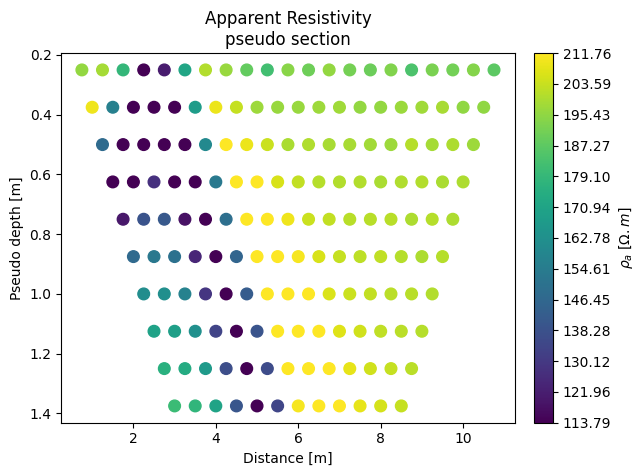
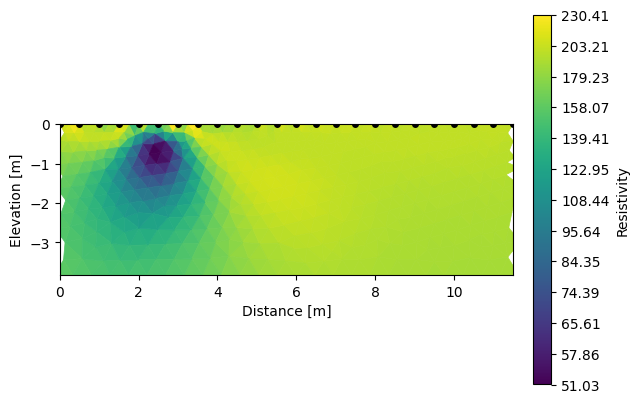
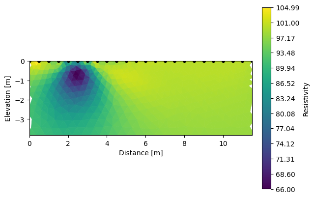
We can already see that the pseudo-section already show clearly the import on the region we defined. We can now invert these apparent resistivities. Inverting the forward models allow the user to see if the parameters of the surveys (the sequence and electrode spacing) were optimium to resolve the target. If needed he can change them and do the whole process again.
[10]:
k.invert()
Writing .in file and protocol.dat... All non fixed parameters reset to 100 Ohm.m and 0 mrad, as the survey to be inverted is from a forward model.
done

--------------------- MAIN INVERSION ------------------


 >> R  2    R e s i s t i v i t y   I n v e r s i o n   v4.10 <<

 >> D a t e : 03 - 12 - 2023
 >> My beautiful survey
 >> I n v e r s e   S o l u t i o n   S e l e c t e d <<
 >> Determining storage needed for finite element conductance matrix
 >> Generating index array for finite element conductance matrix
 >> Reading start resistivity from res0.dat
 >> R e g u l a r i s e d   T y p e <<
 >>   L i n e a r    F i l t e r    <<
 >> L o g - D a t a   I n v e r s i o n <<
 >> N o r m a l   R e g u l a r i s a t i o n <<
 >> D a t a   w e i g h t s   w i l l   b e  m o d i f i e d <<


 Processing dataset   1


 Measurements read:   165     Measurements rejected:     0
   Geometric mean of apparent resistivities:  0.17448E+03

 >> Total Memory required is:          0.003 Gb

   Iteration   1
     Initial RMS Misfit:        23.61       Number of data ignored:     0
     Alpha:        1359.972   RMS Misfit:        3.12  Roughness:        0.995
     Alpha:         631.243   RMS Misfit:        2.18  Roughness:        1.872
     Alpha:         292.997   RMS Misfit:        1.48  Roughness:        2.993
     Alpha:         135.997   RMS Misfit:        1.23  Roughness:        4.157
     Alpha:          63.124   RMS Misfit:        1.31  Roughness:        5.331
     Step length set to   1.00000
     Final RMS Misfit:        1.23
     Attempted to update data weights and caused overshoot
     treating as converged

 Solution converged - Outputing results to file

 Calculating sensitivity map


 Processing dataset   2


 End of data:  Terminating
1/1 results parsed (1 ok; 0 failed)
All ok
[11]:
k.showResults(index=0) # show the initial model
k.showResults(index=1, sens=False) # show the inverted model
ERROR: No sensitivity attribute found

In a nutshell
[12]:
k = Project(typ='R2')

# defining electrode array
x = np.zeros((24, 3))
x[:,0] = np.arange(0, 24*0.5, 0.5)
k.setElec(elec)

# creating mesh
k.createMesh()

# add region
k.addRegion(np.array([[2,-0.3],[2,-2],[3,-2],[3,-0.3],[2,-0.3]]), 50)

# define sequence
k.createSequence([('dpdp1', 1, 10)])

# forward modelling
k.forward(noise=0.0)

# inverse modelling based on forward results
k.invert()

# show the initial and recovered section
k.showResults(index=0) # initial
k.showResults(index=1, sens=False) # recovered
Working directory is: /media/jkl/data/phd/resipy/src/resipy
clearing dirname
Creating triangular mesh...done (1887 elements)
165 quadrupoles generated.
Writing .in file and mesh.dat... done
Writing protocol.dat... done
Running forward model...

 >> R  2    R e s i s t i v i t y   I n v e r s i o n   v4.10 <<

 >> D a t e : 03 - 12 - 2023
 >> My beautiful survey
 >> F o r w a r d   S o l u t i o n   S e l e c t e d <<
 >> Determining storage needed for finite element conductance matrix
 >> Generating index array for finite element conductance matrix
 >> Reading start resistivity from resistivity.dat

 Measurements read:   165     Measurements rejected:     0

 >> Total Memory required is:          0.000 Gb
0/165 reciprocal measurements found.
All ok
/media/jkl/data/phd/resipy/pyenv/lib/python3.10/site-packages/numpy/lib/function_base.py:2458: DeprecationWarning: Conversion of an array with ndim > 0 to a scalar is deprecated, and will error in future. Ensure you extract a single element from your array before performing this operation. (Deprecated NumPy 1.25.)
  res = asanyarray(outputs, dtype=otypes[0])
Forward modelling done.Writing .in file and protocol.dat... All non fixed parameters reset to 100 Ohm.m and 0 mrad, as the survey to be inverted is from a forward model.
done

--------------------- MAIN INVERSION ------------------


 >> R  2    R e s i s t i v i t y   I n v e r s i o n   v4.10 <<

 >> D a t e : 03 - 12 - 2023
 >> My beautiful survey
 >> I n v e r s e   S o l u t i o n   S e l e c t e d <<
 >> Determining storage needed for finite element conductance matrix
 >> Generating index array for finite element conductance matrix
 >> Reading start resistivity from res0.dat
 >> R e g u l a r i s e d   T y p e <<
 >>   L i n e a r    F i l t e r    <<
 >> L o g - D a t a   I n v e r s i o n <<
 >> N o r m a l   R e g u l a r i s a t i o n <<
 >> D a t a   w e i g h t s   w i l l   b e  m o d i f i e d <<


 Processing dataset   1


 Measurements read:   165     Measurements rejected:     0
   Geometric mean of apparent resistivities:  0.93704E+02

 >> Total Memory required is:          0.003 Gb

   Iteration   1
     Initial RMS Misfit:         3.71       Number of data ignored:     0
     Alpha:        1109.630   RMS Misfit:        1.29  Roughness:        0.203
     Alpha:         515.045   RMS Misfit:        0.91  Roughness:        0.379
     Step length set to   1.00000
     Final RMS Misfit:        0.91
     Final RMS Misfit:        1.01

 Solution converged - Outputing results to file

 Calculating sensitivity map


 Processing dataset   2


 End of data:  Terminating
1/1 results parsed (1 ok; 0 failed)
ERROR: No sensitivity attribute found
All ok
[ ]: