This page was generated from jupyter-notebook/nb_Morris.ipynb. Interactive online version:

Global sensitivity analysis

Global sensitivity analysis is a Monte Carlo based method to rank the importance of parameters in a given modelling problem. As opposed to local senstivity analysis, it does not require the construction of the Jacobian, making it a flexible tool to evaluate complex problems.

Global sensitivty analysis is available in mainly uncertainty quantificaiton packages, as well as some flow and transport programs (e.g. iTOUGH2). GSA is also very popular in catchment modelling and civil engineering/risk analysis problems.

Some GSA work in hydrogeophysics (mainly by Berkeley Lab):

coupled hydrological-thermal-geophysical inversion (Tran et al 2017) > Nicely show how to simplify (i.e. reduce the number of parameters) for a very complex, highly coupled problem
making sense of global senstivity analysis (Wainwright et al 2014) > Very good review article
Sensitivity analysis of environmental models (Pianosi et al 2014) > A systematic review, includes GLUE and RSA
hydrogeology of a nuclear site in the Paris Basin (Deman et al 2016) > A different GSA method was used instead here to look at the low probability breakthrough events
Global Sensitivity and Data-Worth Analyses in iTOUGH2 User’s Guide (Wainwright et al 2016) > An useful manual if you want to learn about the details of setting up a probllem.

In this tutorial, we will see how to link the ResIPy API and SALib for senstivity analysis. Two key elements of SA are (i) forward modelling (Monte Carlo runs) and (ii) specifying the parameter ranges. This notebook will showcase of the use of the Method of Morris, which is known for its relatively small computational cost. This tutorial is modified from the one posted on https://github.com/SALib/SATut to demonstrate its coupling with ResIPy

Morris sensitivity method

The Morris one-at-a-time (OAT) method (Morris, 1991) can be considered as an extension of the local sensitivity method. Each parameter range is scaled to the unit interval [0, 1] and partitioned into \((p−1)\) equally-sized intervals. The reference value of each parameter is selected randomly from the set \({0, 1/(p−1), 2/(p−1), …, 1−Δ}\). The fixed increment \(Δ=p/{2(p−1)}\) is added to each parameter in random order to compute the elementary effect (\(EE\)) of \(x_i\)

\[ \begin{align}\begin{aligned}EE_i=\frac{1}{\tau_y}\frac{f(x_1*,...,x_i*+\Delta,...,x_k*)-f(x_1*,...,x_k*)}{\Delta}\\where :math:`{x_i⁎}` is the randomly selected parameter set, and τy is the output-scaling factor. To compute EEi for k parameters, we need (k+1) simulations (called one “path”) in the same way as that of the local sensitivity method. By having multiple paths, we have an ensemble of EEs for each parameter. The total number of simulations is r(k+1), where r is the number of paths.\end{aligned}\end{align} \]

We compute three statistics: the mean \(EE\), standard deviation (STD) of \(EE\), and mean of absolute \(EE\). * mean EE (:math:`mu`) represents the average effect of each parameter over the parameter space, the mean EE can be regarded as a global sensitivity measure. * mean |EE| (:math:`mu*`) is used to identify the non-influential factors, * STD of EE (:math:`sigma`) is used to identify nonlinear and/or interaction effects. (The standard error of mean (SEM) of EE, defined as \(SEM=STD/r^{0.5}\), is used to calculate the confidence interval of mean EE (Morris, 1991))

This cell is copied from (Wainwright et al 2014)

Importing libraries

[13]:

import warnings
warnings.filterwarnings('ignore')
import os
import sys
sys.path.append('../src') # add here the relative path of the API folder
from resipy import Project
import numpy as np # numpy for electrode generation
import pandas as pd
from IPython.utils import io  # suppress R2 outputs during MC runs

The SALib package

SALib is a free open-source Python library

If you use Python, you can install it by running the command

pip install SALib

Documentation is available online and you can also view the code on Github.

The library includes: * Sobol Sensitivity Analysis (Sobol 2001, Saltelli 2002, Saltelli et al. 2010) * Method of Morris, including groups and optimal trajectories (Morris 1991, Campolongo et al. 2007) * Fourier Amplitude Sensitivity Test (FAST) (Cukier et al. 1973, Saltelli et al. 1999) * Delta Moment-Independent Measure (Borgonovo 2007, Plischke et al. 2013) * Derivative-based Global Sensitivity Measure (DGSM) (Sobol and Kucherenko 2009) * Fractional Factorial Sensitivity Analysis (Saltelli et al. 2008)

SALib Tutorial

[2]:

# import the packages
from SALib.sample import morris as ms
from SALib.analyze import morris as ma
from SALib.plotting import morris as mp

Create ERT forward problem with ResIPy

In the code below, created a Project forward problem to be analyzed

[3]:

k = Project(typ='R2')

elec = np.zeros((24,3))
elec[:,0] = np.arange(0, 24*0.5, 0.5) # with 0.5 m spacing and 24 electrodes
k.setElec(elec)
#print(k.elec)

# defining electrode array
x = np.zeros((24, 3))
x[:,0] = np.arange(0, 24*0.5, 0.5)
k.setElec(elec)

# creating mesh
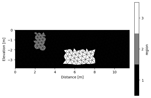
k.createMesh(res0=20)

# add region
k.addRegion(np.array([[2,-0.3],[2,-2],[3,-2],[3,-0.3],[2,-0.3]]), 50)
k.addRegion(np.array([[5,-2],[5,-3.5],[8,-3.5],[8,-2],[5,-2]]), 500)

# define sequence
k.createSequence([('dpdp1', 1, 10)])

# forward modelling
k.forward(noise=0.025)

# read results
fwd_dir = os.path.relpath('../src/resipy/invdir/fwd')

obs_data = np.loadtxt(os.path.join(fwd_dir, 'R2_forward.dat'),skiprows =1)
obs_data = obs_data[:,6]

# plot
k.showMesh()

Working directory is: /media/jkl/data/phd/resipy/src/resipy
clearing dirname
Creating triangular mesh...done (1887 elements)
165 quadrupoles generated.
Writing .in file and mesh.dat... done
Writing protocol.dat... done
Running forward model...

 >> R  2    R e s i s t i v i t y   I n v e r s i o n   v4.10 <<

 >> D a t e : 03 - 12 - 2023
 >> My beautiful survey
 >> F o r w a r d   S o l u t i o n   S e l e c t e d <<
 >> Determining storage needed for finite element conductance matrix
 >> Generating index array for finite element conductance matrix
 >> Reading start resistivity from resistivity.dat

 Measurements read:   165     Measurements rejected:     0

 >> Total Memory required is:          0.000 Gb
0/165 reciprocal measurements found.
Forward modelling done.

All ok
/media/jkl/data/phd/resipy/pyenv/lib/python3.10/site-packages/numpy/lib/function_base.py:2458: DeprecationWarning: Conversion of an array with ndim > 0 to a scalar is deprecated, and will error in future. Ensure you extract a single element from your array before performing this operation. (Deprecated NumPy 1.25.)
  res = asanyarray(outputs, dtype=otypes[0])

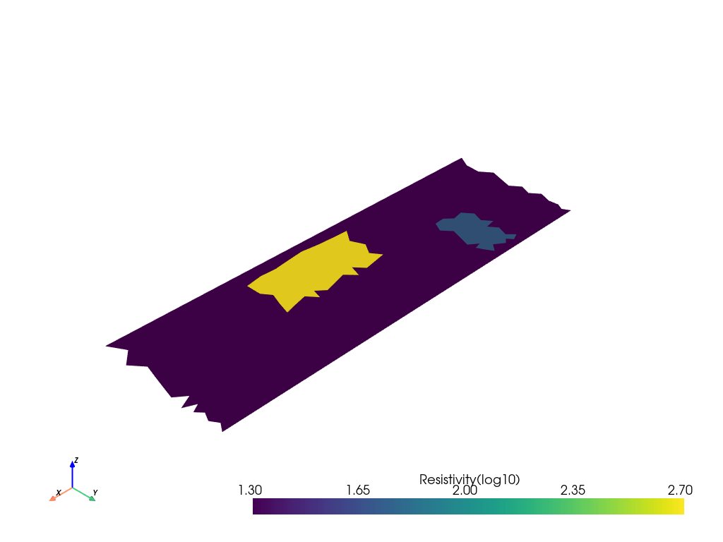
Option to view resistivity fields with pyvista

[4]:

import pyvista as pv
mesh = pv.read(os.path.join(fwd_dir, 'forward_model.vtk'))
mesh.plot(scalars='Resistivity(log10)',notebook=True)
mesh

[4]:

Header

Data Arrays

UnstructuredGrid	Information
N Cells	893
N Points	496
X Bounds	-1.400e-01, 1.168e+01
Y Bounds	-3.830e+00, 0.000e+00
Z Bounds	0.000e+00, 0.000e+00
N Arrays	2

Name	Field	Type	N Comp	Min	Max
Resistivity(ohm.m)	Cells	float64	1	2.000e+01	5.000e+02
Resistivity(log10)	Cells	float64	1	1.301e+00	2.699e+00

[5]:

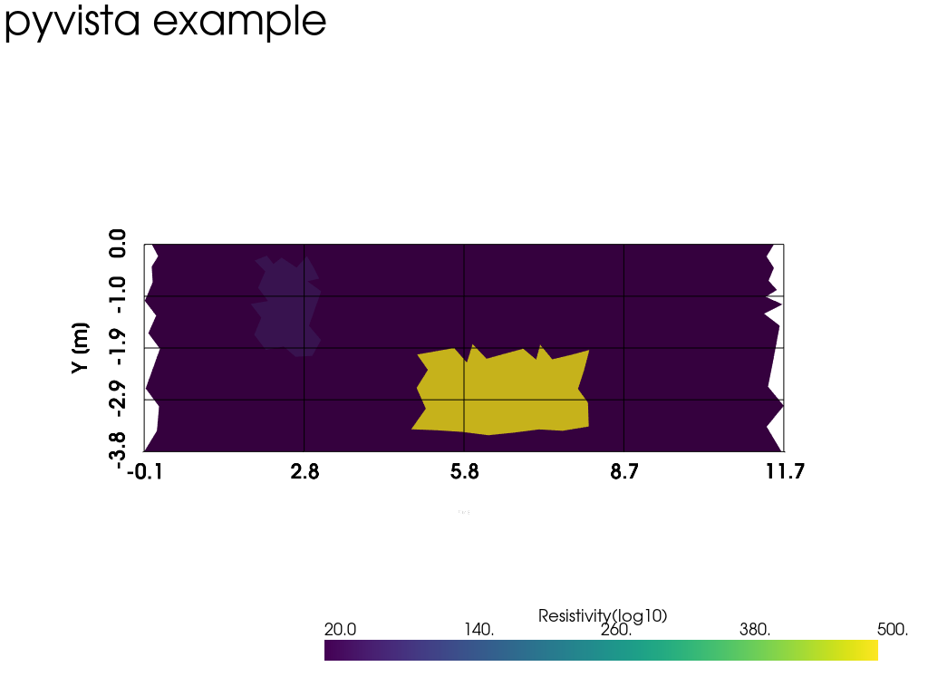
import pyvista as pv

plotter = pv.Plotter()
mesh = pv.read(os.path.join(fwd_dir, 'forward_model.vtk'))

plotter.add_mesh(mesh,cmap="viridis" ,stitle="Resistivity(log10)") #scalars='Resistivity(log10)'
#plotter.show_axes()

_ = plotter.show_bounds(grid='front', location='outer', all_edges=True, xlabel="X [m]",ylabel="Y [m]")
plotter.add_text('pyvista example')
#plotter.update_scalar_bar_range([-2000,2000], name="Resistivity(log10)")

#plotter.add_mesh(mesh, cmap="bone", opacity="linear", stitle="Linear Opacity")
plotter.view_xy()
plotter.show()
#plotter.show(screenshot='test.png')

Define a problem file

In the code below, a problem file is used to define the parameters and their ranges we wish to explore, which corresponds to the following table:

Parameter	Range	Description
rho0 [ohm m]	10 [1]	background
rho1 [ohm m]	10 [2]	inclusion A
rho2 [ohm m]	10 [3]	inclusion B

[6]:

morris_problem = {
    'num_vars': 3,
    # These are their names
    'names': ['rho1', 'rho2', 'rho3'], # can add z1 z2 etc.
    # Plausible ranges over which we'll move the variables
    'bounds': [[0.5,3.5], # log10 of rho (ohm m)
               [0.5,3.5],
               [0.5,3.5]#,
   #            [-3,-1],
   #            [-7,-4],
              ],
    # I don't want to group any of these variables together
    'groups': None
    }

Generate a Sample

We then generate a sample using the morris.sample() procedure from the SALib package.

[7]:

number_of_trajectories = 20
sample = ms.sample(morris_problem, number_of_trajectories, num_levels=10)
len(sample)
print(sample[79,:])

[1.16666667 1.5        1.83333333]

Run the sample through the monte carlo procedure in R2

Great! You have defined your problem and have created a series of input files for forward runs. Now you need to run R2 for each of them to obtain their ERT responses.

For this example, each sample takes a few seconds to run on a PC.

[8]:

#%%capture
simu_ensemble = np.zeros((len(obs_data),len(sample)))
for ii in range(0, len(sample)):
    with io.capture_output() as captured:          # suppress inline output from ResIPy
        # creating mesh
        k.createMesh(res0=10**sample[ii,0])   # need to use more effective method, no need to create mesh every time

        # add region
        k.addRegion(np.array([[2,-0.3],[2,-2],[3,-2],[3,-0.3],[2,-0.3]]), 10**sample[ii,1])
        k.addRegion(np.array([[5,-2],[5,-3.5],[8,-3.5],[8,-2],[5,-2]]), 10**sample[ii,2])

        # forward modelling
        k.forward(noise=0.025, iplot = False)
        out_data = np.loadtxt(os.path.join(fwd_dir, 'R2_forward.dat'),skiprows =1)
        simu_ensemble[:,ii] = out_data[:,6]
    print("Running sample",ii+1)

All ok

Running sample 1

All ok

Running sample 2

All ok

Running sample 3

All ok

Running sample 4

All ok

Running sample 5

All ok

Running sample 6

All ok

Running sample 7

All ok

Running sample 8

All ok

Running sample 9

All ok

Running sample 10

All ok

Running sample 11

All ok

Running sample 12

All ok

Running sample 13

All ok

Running sample 14

All ok

Running sample 15

All ok

Running sample 16

All ok

Running sample 17

All ok

Running sample 18

All ok

Running sample 19

All ok

Running sample 20

All ok

Running sample 21

All ok

Running sample 22

All ok

Running sample 23

All ok

Running sample 24

All ok

Running sample 25

All ok

Running sample 26

All ok

Running sample 27

All ok

Running sample 28

All ok

Running sample 29

All ok

Running sample 30

All ok

Running sample 31

All ok

Running sample 32

All ok

Running sample 33

All ok

Running sample 34

All ok

Running sample 35

All ok

Running sample 36

All ok

Running sample 37

All ok

Running sample 38

All ok

Running sample 39

All ok

Running sample 40

All ok

Running sample 41

All ok

Running sample 42

All ok

Running sample 43

All ok

Running sample 44

All ok

Running sample 45

All ok

Running sample 46

All ok

Running sample 47

All ok

Running sample 48

All ok

Running sample 49

All ok

Running sample 50

All ok

Running sample 51

All ok

Running sample 52

All ok

Running sample 53

All ok

Running sample 54

All ok

Running sample 55

All ok

Running sample 56

All ok

Running sample 57

All ok

Running sample 58

All ok

Running sample 59

All ok

Running sample 60

All ok

Running sample 61

All ok

Running sample 62

All ok

Running sample 63

All ok

Running sample 64

All ok

Running sample 65

All ok

Running sample 66

All ok

Running sample 67

All ok

Running sample 68

All ok

Running sample 69

All ok

Running sample 70

All ok

Running sample 71

All ok

Running sample 72

All ok

Running sample 73

All ok

Running sample 74

All ok

Running sample 75

All ok

Running sample 76

All ok

Running sample 77

All ok

Running sample 78

All ok

Running sample 79
Running sample 80

All ok

Factor Prioritisation

We’ll run a sensitivity analysis of the power module to see which is the most influential parameter.

The results parameters are called mu, sigma and mu_star.

Mu is the mean effect caused by the input parameter being moved over its range.
Sigma is the standard deviation of the mean effect.
Mu_star is the mean absolute effect.

The higher the mean absolute effect for a parameter, the more sensitive/important it is*

[9]:

# Define an objective function: here I use the error weighted rmse
def obj_fun(sim,obs,noise):
    y = np.divide(sim-obs,noise)   # weighted data misfit
    y = np.sqrt(np.inner(y,y))
    return y

output = np.zeros((1,len(sample)))
for ii in range(0, len(sample)):
    output[0,ii] = obj_fun(simu_ensemble[:,ii],obs_data,0.025*obs_data)    # assume 2.5% noise in the data

# Store the results for plotting of the analysis
Si = ma.analyze(morris_problem, sample, output, print_to_console=False)
print("{:20s} {:>7s} {:>7s} {:>7s}".format("Name", "mean(EE)", "mean(|EE|)", "std(EE)"))
for name, s1, st, mean in zip(morris_problem['names'],
                              Si['mu'],
                              Si['mu_star'],
                              Si['sigma']):
    print("{:20s} {:=7.3f} {:=7.3f} {:=7.3f}".format(name, s1, st, mean))

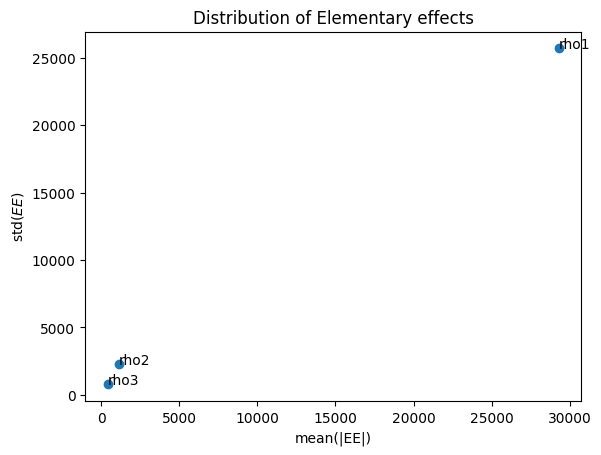
Name                 mean(EE) mean(|EE|) std(EE)
rho1                 29271.700 29271.700 25700.482
rho2                 1133.239 1146.483 2255.792
rho3                 413.524 428.156 766.059

[10]:

# make a plot
import matplotlib.pyplot as plt
import numpy as np
fig, ax = plt.subplots()
ax.scatter(Si['mu_star'],Si['sigma'])
#ax.plot(Si['mu_star'],2*Si['sigma']/np.sqrt(number_of_trajectories),'--',alpha=0.5)
#ax.plot(np.array([0,Si['mu_star'][0]]),2*np.array([0,Si['sigma'][0]/np.sqrt(number_of_trajectories)]),'--',alpha=0.5)

plt.title('Distribution of Elementary effects')
plt.xlabel('mean(|EE|)')
plt.ylabel('std($EE$)')
for i, txt in enumerate(Si['names']):
    ax.annotate(txt, (Si['mu_star'][i], Si['sigma'][i]))

# higher mean |EE|, more important factor
# line within the dashed envelope means nonlinear or interaction effects dominant

Summary

Sensitivity analysis helps you:

Think through your assumptions
Quantify uncertainty
Focus on the most influential uncertainties first

Learn Python

Similar packages to SALib for other languages/programmes:

Matlab Toolbox SAFE for GSA
‘sensitivity’ package for R (Michael Tso used it for GSA in his leak detection paper)

[11]:

# run this so that a navigation sidebar will bee generated when exporting this notebook as HTML
#%%javascript
#$('<div id="toc"></div>').css({position: 'fixed', top: '120px', left: 0}).appendTo(document.body);
#$.getScript('https://kmahelona.github.io/ipython_notebook_goodies/ipython_notebook_toc.js');

[12]:

help(k.addRegion)

Help on method addRegion in module resipy.Project:

addRegion(xz, res0=100, phase0=1, blocky=False, fixed=False, ax=None, iplot=False) method of resipy.Project.Project instance
    Add region according to a polyline defined by `xz` and assign it
    the starting resistivity `res0`.

    Parameters
    ----------
    xz : array
        Array with two columns for the x and y coordinates.
    res0 : float, optional
        Resistivity values of the defined area.
    phase0 : float, optional
        Read only if you choose the cR2 option. Phase value of the defined
        area in mrad
    blocky : bool, optional
        If `True` the boundary of the region will be blocky if inversion
        is block inversion.
    fixed : bool, optional
        If `True`, the inversion will keep the starting resistivity of this
        region.
    ax : matplotlib.axes.Axes
        If not `None`, the region will be plotted against this axes.
    iplot : bool, optional
        If `True` , the updated mesh with the region will be plotted.